Quantization Strategies: Mastering the Bit-Budget
A standard ResNet-50 model takes roughly 100MB of memory and 20-30ms of GPU time in FP32. For a high-end desktop, that is fine. For a battery-powered VR headset or a mobile phone, it is a disaster.
Quantization is the process of reducing the precision of your model’s weights and activations. By moving from 32-bit floats to 8-bit (or even 4-bit) integers, we can achieve a 4x size reduction and up to a 10x speedup on hardware with specialized integer units.
In this chapter, we will move beyond the basics and look at the rigorous mathematics of quantization, learning how to shrink a model without destroying its "intelligence."
The Maturity of Quantization: From Floats to Bits
You have built your inference engine, verified its correctness in FP32, and optimized your loops. But then you look at your binary size: 100MB for a single ResNet-50 model. You look at your frame time on a mobile device: 100ms. You look at your battery drain: massive.
Quantization is the process of reducing the precision of your model’s weights and activations. By moving from 32-bit floats to 8-bit (or even 4-bit) integers, we achieve three critical production goals: 1. 4x Memory Reduction: A 100MB model becomes 25MB. 2. 4x Bandwidth Savings: The "Memory Wall" is pushed back because we move fewer bytes per operation. 3. 10x Speedup: Specialized hardware (like DP4A or Tensor Cores) can process multiple integers in the time it takes to process one float.
In this chapter, we move from "understanding quantization" to "performing quantization." We will explore both the Pragmatic Path (using ONNX Runtime’s toolchain) and the Educational Path (implementing custom integer shaders in Vulkan).
The Intuition: Signal vs. Noise
Why does quantization work? Why don’t neural networks stop working when we throw away 75% of their numerical precision?
Neural networks are inherently Robust to Noise. During training, we use techniques like Dropout and Weight Decay that intentionally "mess with" the data. The network learns to find high-level patterns (the signal) and ignore the tiny details (the noise). Quantization is essentially adding a very specific type of "rounding noise." As long as that noise is smaller than the signal required to distinguish a "Dog" from a "Cat," the network functions perfectly.
Think of it like a digital photograph. An uncompressed RAW file (FP32) has millions of colors you can’t even see. A JPEG (INT8) reduces that detail, but to the human eye, the image looks identical.
The Mathematical Foundation: Floating Point to Integer
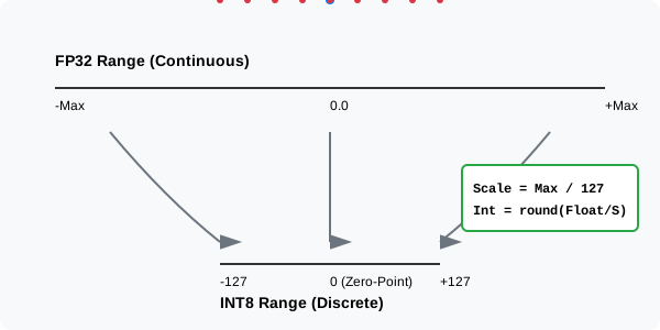
Quantization is a mapping function that squashes a continuous infinite range of real numbers into a small, discrete set of integers.
1. Symmetric Quantization (The Speed King)
This is the simplest and fastest form. We assume the data is centered at zero. We map the range ] to the integer range ] (for signed 8-bit).
-
Pros: Extremely fast math. Because there is no "offset," the hardware can perform pure integer dot products ( ).
-
Cons: If your data is heavily skewed (e.g., all values are between 10 and 20), symmetric quantization is wasteful. You’ll use only a tiny sliver of the available integer range.
2. Asymmetric Quantization (The Accuracy King)
This is what you use when your data is shifted or mostly positive (like ReLU activations). We map the range ] to the unsigned integer range ].
Where is the Zero-Point. It ensures that the floating-point value 0.0 maps perfectly to an integer. This is critical because neural networks use "Zero" to represent missing data or padded edges. If 0.0 became 0.3, the network would see "signal" where there should be "silence."
Fixed-Point Arithmetic: Doing Math in 8-bit
Here is the secret: Once you have integers, you do not convert them back to floats to do math. You do the math in integers and only "rescale" at the very end of the layer. This is how we achieve the speedup on integer-optimized hardware.
Imagine a matrix multiplication . In quantized space, this becomes:
The Integer Rescale Trick
In your Vulkan shader, the is performed using 32-bit integer accumulators to prevent overflow. To get the final INT8 result for the next layer, we must rescale the 32-bit sum back down.
Mathematically, we want to compute:
Since floating-point multiplication is slow, we pre-calculate the constant and represent it as a Fixed-Point Multiplier (a large integer) and a Bit-Shift. In your shader, the "Rescale" becomes a single integer multiply and a right-shift ( ), which is significantly faster than any float operation.
The ONNX Runtime Quantization Workflow (The Pragmatic Path)
If you are using ONNX Runtime in your Vulkan app (as taught in the Third-Party Libraries chapter), you don’t need to write the math yourself. You use the ONNX Runtime Quantization Toolchain.
Step 1: Choosing Your Strategy
You must choose between Dynamic and Static quantization.
-
Dynamic Quantization:
-
How: Weights are quantized offline. Activations are quantized at runtime by the engine.
-
Pros: No dataset required. Easy to use.
-
Best for: LSTMs, Transformers, and CPU-bound inference.
-
-
Static Quantization (PTQ):
-
How: Both weights and activations are quantized offline.
-
Pros: Fastest possible performance. Allows the GPU to use specialized INT8 instructions.
-
Requirements: Requires a small Calibration Dataset (100-500 images) to "learn" the range of activations.
-
Step 2: Implementing a Calibration Data Reader
To perform Static Quantization, the tool needs to know what "normal" data looks like so it can find the optimal scale factors. You provide this via a CalibrationDataReader.
import numpy as np
import onnxruntime
from onnxruntime.quantization import CalibrationDataReader

class ImageNetDataReader(CalibrationDataReader):
    def __init__(self, calibration_image_folder, input_name):
        self.image_folder = calibration_image_folder
        self.input_name = input_name
        self.data_iter = None
        self.preprocessed_data = []
        self.preprocess_images()

    def preprocess_images(self):
        # Load 100-200 images for a good statistical sample.
        # CRITICAL: This MUST match your C++ preprocessing (Mean/StdDev) exactly!
        for img_path in list_images(self.image_folder)[:100]:
            img = load_image(img_path)
            img = resize_aspect_aware(img, (224, 224))
            # ImageNet Normalization
            img = (img / 255.0 - [0.485, 0.456, 0.406]) / [0.229, 0.224, 0.225]
            img = img.transpose(2, 0, 1) # HWC to NCHW
            img = np.expand_dims(img, axis=0).astype(np.float32)
            self.preprocessed_data.append({self.input_name: img})

    def get_next(self):
        if self.data_iter is None:
            self.data_iter = iter(self.preprocessed_data)
        return next(self.data_iter, None)
Step 3: The Quantization Script
With your reader ready, you run the quantization process. This script will produce a .quant.onnx file that is 4x smaller than your original.
from onnxruntime.quantization import quantize_static, QuantType, QuantFormat

model_fp32 = "models/mobilenetv2.onnx"
model_int8 = "models/mobilenetv2.quant.onnx"

# Create our data reader
dr = ImageNetDataReader("data/calibration_images", "input")

# Run the quantization
quantize_static(
    model_fp32,
    model_int8,
    dr,
    quant_format=QuantFormat.QDQ, # Quantize-Dequantize format (modern ORT standard)
    per_channel=True,             # High precision for depthwise convs
    weight_type=QuantType.QInt8,
    activation_type=QuantType.QInt8,
    nodes_to_exclude=[]           # Add names of sensitive layers here if needed
)
print(f"Quantized model saved to {model_int8}")
Step 4: Loading in C++ and Enabling Acceleration
Loading a quantized model in your Vulkan C++ app is identical to loading an FP32 model. However, to get the speedup, you must ensure your SessionOptions are configured to use a provider that supports INT8 hardware instructions.
Ort::SessionOptions sessionOptions;

// 1. Enable Graph Optimizations
sessionOptions.SetGraphOptimizationLevel(GraphOptimizationLevel::ORT_ENABLE_ALL);

// 2. Append the WebGPU or DirectML provider
// These providers will detect the INT8 nodes and map them to DP4A/Tensor Core instructions
sessionOptions.AppendExecutionProvider("webgpu");

// 3. Load the quantized model
Ort::Session session(env, L"models/mobilenetv2.quant.onnx", sessionOptions);
How do you know it’s working?
If you look at the ONNX Runtime logs (set ORT_LOGGING_LEVEL_VERBOSE), you should see messages like Placing node … on DML_Execution_Provider. If you see nodes staying on the CPU_Execution_Provider, it means your hardware doesn’t support the required INT8 operations or the driver is out of date.
Transitioning: Mixed-Precision Inference
Quantization isn’t all-or-nothing. Sometimes, quantizing the entire model results in too much accuracy loss. Professional engines use Mixed-Precision.
-
Sensitive Layers: Early layers (which see raw pixels) or late layers (which produce probabilities) are often kept in FP16 or FP32 to preserve precision.
-
Bottleneck Layers: The middle 80% of the network (the expensive convolutions) are quantized to INT8.
Excluding Fragile Nodes
In the quantize_static call, use the nodes_to_exclude parameter. You can find the node names using a tool like Netron.
# Example: Keep the final classifier head in FP32
quantize_static(..., nodes_to_exclude=['Classifier_Head_FC'])
If your model’s accuracy drops from 95% to 70%, try excluding the final layer—this often restores 90% of the lost accuracy with almost no performance penalty.
Debugging Quantized Models: The Hunt for Error
When a quantized model fails, it doesn’t crash; it just gives the wrong answer. This is the "Silent Accuracy Bug."
-
Cosine Similarity: Compare the activations of your FP32 model vs. your INT8 model layer-by-layer.
-
: Perfect quantization.
-
: High distortion. This layer is a candidate for exclusion.
-
-
Sensitivity Analysis: Use the
onnxruntime.quantization.api.quantizesensitivity analysis tools to automatically identify which layers contribute most to accuracy loss. -
Visualizing Clipping: If your calibration histogram shows that 10% of your data is being "clipped" (pushed to 127), your scale factor is too small. Use a different Calibration Method (e.g.,
EntropyorPercentileinstead ofMinMax).
Hardware Compatibility: Why INT8 isn’t always faster
Before you ship a quantized model, verify your user’s hardware capabilities.
-
Modern GPUs (NVIDIA Turing+, AMD RDNA3+, Intel Xe): Feature dedicated INT8 units. Quantization provides a boost.
-
Older GPUs: Might lack specialized integer math. On these chips, the GPU has to "emulate" INT8 using FP32, which can actually be slower due to the packing/unpacking overhead.
-
The Pro Move: Ship both the FP32 and INT8 models. Use Vulkan to query
VkPhysicalDeviceFeaturesat runtime. IfshaderInt8is supported, load the quantized model; otherwise, fall back to the float version.
Calibration: Finding the Clipping Threshold
You cannot just use the absolute of your weights to find the scale. If 99.9% of your weights are between -1 and 1, but one single outlier is at 50, your scale will be huge, and you’ll lose all precision for the important 99.9%.
The K-L Divergence Strategy
Professional engines use K-L Divergence (Kullback–Leibler) to find the optimal clipping threshold.
-
Collect: Run 100-500 real images through your model and record the distribution (histogram) of activations for every layer.
-
Search: Try different clipping values (e.g., clipping the range at 2.0, then 2.5, then 3.0).
-
Compare: Quantize the clipped data, then dequantize it. Compare this "distorted" distribution back to the original FP32 distribution.
-
Pick: Select the threshold that minimizes the Information Loss. Often, throwing away 0.1% of outlier values results in 10x better precision for the remaining 99.9%.
PTQ vs. QAT: The Deployment Choice
When you decide to quantize, you must choose between two workflows:
-
Post-Training Quantization (PTQ):
-
The Process: Take an existing FP32 model and apply calibration.
-
Pros: Fast (takes minutes), easy to use, no retraining required.
-
Cons: Can result in significant accuracy loss for "sensitive" models (like object detectors).
-
-
Quantization-Aware Training (QAT):
-
The Process: You inject "Fake Quantization" nodes into your PyTorch graph and continue training for a few epochs. The network learns to adjust its weights to be robust to rounding errors.
-
Pros: High accuracy (often matches FP32 perfectly).
-
Cons: Slow (requires a training setup, GPU time, and a labeled dataset).
-
The Expert Recommendation: Start with PTQ. Only if the accuracy drop is more than 1% should you invest the time in QAT.
Granularity: Per-Tensor vs. Per-Channel
The "Scale" is the most precious number in quantization. How you calculate it determines your accuracy.
-
Per-Tensor (Global):
-
You calculate one scale for the entire weight buffer of a layer.
-
Pros: Simplest to implement. Minimal memory overhead (one float per layer).
-
Cons: If one output filter has weights in the range [-10, 10] and another has [ -0.1, 0.1], the global scale will be biased toward the large filter. The small filter will be crushed to zero, losing all its feature-detecting power.
-
-
Per-Channel (Standard):
-
You calculate a unique scale for every output filter (channel).
-
Pros: Preserves the unique dynamic range of every feature. This is mandatory for modern architectures like MobileNetV2 that use Depthwise Convolutions.
-
Cons: Slightly more complex shader math (you must index into a scale buffer).
-
Hardware Acceleration: DP4A and the dotProduct Extension
Why is INT8 actually faster? It’s not just about smaller numbers; it’s about Vector Throughput.
Modern GPUs feature instructions designed for "Horizontal" math. In a standard multiply-add, one thread does one operation. With DP4A (Dot Product 4-way Accumulate), one thread can process four pairs of 8-bit integers in a single clock cycle.
The Instruction: dotProduct4x8bitPackedEXT
This instruction takes two 32-bit registers, treats each as four 8-bit integers, multiplies them, and adds the result to an accumulator.
// Logic of the instruction
int dotProduct4x8bitPackedEXT(uint a, uint b, int acc) {
    int res = acc;
    res += int8_t(a & 0xFF) * int8_t(b & 0xFF);
    res += int8_t((a >> 8) & 0xFF) * int8_t((b >> 8) & 0xFF);
    res += int8_t((a >> 16) & 0xFF) * int8_t((b >> 16) & 0xFF);
    res += int8_t((a >> 24) & 0xFF) * int8_t((b >> 24) & 0xFF);
    return res;
}
By using this, your compute shader moves from being a "one-at-a-time" calculator to a "batch processor," potentially increasing your arithmetic throughput by instantly.
Advanced: 4-Bit Quantization (INT4) and Grouped Stats
In the era of Large Language Models (LLMs), even 8-bit is sometimes too large. We are now seeing a shift to INT4.
-
Grouped Quantization: Instead of one scale per channel, we use one scale for every 32 or 64 weights. This handles the "locality" of weights in huge models.
-
Storage: Two 4-bit weights are packed into a single byte.
-
Math: Since most GPUs don’t have native 4-bit math units yet, we use De-quantize on Load.
-
The GPU reads the 4-bit weight from VRAM (saving bandwidth).
-
The shader immediately converts it to
float16orint8. -
The math proceeds as normal.
-
The Benefit: You are almost always "Memory Bound" in LLMs. Reducing weight size by compared to FP32 provides a speedup, even if the math itself isn’t faster.
The Next Frontier: Weight Sparsity
Quantization reduces the Precision of weights. Sparsity reduces the Number of weights.
Neural networks are often "over-parameterized." Many weights are so close to zero that they have no effect on the output.
-
Unstructured Sparsity: You set individual small weights to zero.
-
Problem: GPUs hate "random" zeros. It creates branch divergence and uncoalesced memory access.
-
-
Structured Sparsity (2:4): NVIDIA Ampere GPUs introduced hardware support for 2:4 Sparsity.
-
The Rule: In every block of 4 weights, at least 2 must be zero.
-
The Benefit: The GPU hardware "skips" the zero multiplications, providing a throughput boost on top of any quantization gains.
-
When you combine INT8 Quantization with 2:4 Sparsity, you can achieve a speedup over a naive FP32 implementation.
Hands-on: Implementing Your First Quantized Layer (The Educational Path)
Let’s build a Symmetric Per-Channel Quantized Convolution pipeline from scratch. This is the path you take when you want full control over your Vulkan inference engine.
Phase 1: Offline Weight Preparation (C++)
Before your app starts, you must transform your float32 weights. We will calculate the scale factors and pack the weights into a byte array.
struct QuantizedLayer {
    std::vector<int8_t> weights; // INT8 weights
    std::vector<float> rescaleFactors; // Pre-calculated (S_in * S_w) / S_out
    int32_t bias_scale; // Usually quantized to 32-bit
};

QuantizedLayer quantizeWeights(const float* fp32Weights, uint32_t outC, uint32_t inC, uint32_t kSize, float inputScale, float outputScale) {
    QuantizedLayer layer;
    uint32_t filterSize = inC * kSize * kSize;
    layer.weights.resize(outC * filterSize);
    layer.rescaleFactors.resize(outC);

    for (uint32_t oc = 0; oc < outC; ++oc) {
        // 1. Find max for this channel
        float maxW = 0.0f;
        for (uint32_t i = 0; i < filterSize; ++i) {
            maxW = std::max(maxW, std::abs(fp32Weights[oc * filterSize + i]));
        }

        // 2. Calculate Weight Scale
        float weightScale = maxW / 127.0f;

        // 3. Pre-calculate the Rescale Factor for the shader
        // This moves the floating point division out of the hot loop
        layer.rescaleFactors[oc] = (inputScale * weightScale) / outputScale;

        // 4. Quantize Weights
        for (uint32_t i = 0; i < filterSize; ++i) {
            float v = fp32Weights[oc * filterSize + i] / weightScale;
            layer.weights[oc * filterSize + i] = static_cast<int8_t>(std::clamp(std::round(v), -127.0f, 127.0f));
        }
    }
    return layer;
}
Phase 2: Vulkan Pipeline Configuration
Quantized shaders require specific buffer layouts. You are no longer moving float arrays; you are moving uint8_t (packed) arrays.
-
Buffer Storage: Use
VK_BUFFER_USAGE_STORAGE_BUFFER_BIT. -
Descriptor Set:
-
Binding 0: Input Activations (INT8) -
Binding 1: Weights (INT8) -
Binding 2: Rescale Factors (FP32 - One per channel) -
Binding 3: Output Activations (INT8)
-
Phase 3: The Optimized INT8 Shader
We will use the dotProduct4x8bitPackedEXT instruction. This requires the GL_EXT_shader_dot_product extension.
#version 450
#extension GL_EXT_shader_dot_product : require
#extension GL_EXT_shader_explicit_arithmetic_types_int8 : require

layout(local_size_x = 16, local_size_y = 16) in;

layout(std430, set = 0, binding = 0) buffer Input  { uint  inData[]; };
layout(std430, set = 0, binding = 1) buffer Weight { uint  wData[];  };
layout(std430, set = 0, binding = 2) buffer Factors { float rescale[]; };
layout(std430, set = 0, binding = 3) buffer Output { uint  outData[]; };

void main() {
    uint outC = gl_GlobalInvocationID.z;
    ivec2 pos = ivec2(gl_GlobalInvocationID.xy);

    // 1. Initialize 32-bit Accumulator
    int sum = 0;

    // 2. The Vectorized Hot Loop
    // We process 4 channels at a time using a single instruction
    for(uint i = 0; i < (inputChannels / 4); ++i) {
        uint a = inData[idx_in + i];
        uint b = wData[idx_w + i];
        sum = dotProduct4x8bitPackedEXT(a, b, sum);
    }

    // 3. The Fixed-Point Rescale
    // We bring the high-precision sum back to the 8-bit range of the next layer
    float result = float(sum) * rescale[outC];

    // 4. Re-pack into the output buffer
    // Note: In a real shader, you would collect 4 results and write one 'uint'
    store_packed_result(pos, outC, int8_t(clamp(round(result), -128, 127)));
}
Implementation Checklist: The "Gotchas"
-
Alignment: Your input channels must be a multiple of 4 to use
dp4a. If they aren’t, you must pad your tensors with zeros. -
Zero-Point: In this example, we used Symmetric quantization (zero-point = 0). If you use Asymmetric (needed for ReLU), your math becomes . This requires an extra subtraction in the loop, which can reduce performance.
-
Intermediate Overflow: Ensure your
sumdoesn’t exceed . For most 8-bit models, this is safe for up to 16,384 channels.
Summary: The Quantization Roadmap
Quantization is the "Superpower" of ML deployment. It allows you to run models on hardware that would otherwise be impossible.
-
The Pragmatic Path: Use the ONNX Runtime Quantization Toolchain. Implement a
CalibrationDataReaderto capture activation ranges, runquantize_static, and load the.quant.onnxfile in your app. It handles the math, the hardware mapping, and the optimizations for you. -
The Educational Path: Build custom INT8 shaders using
dotProduct4x8bitPackedEXT. Master the Fixed-Point Rescale trick to keep your math in integers as long as possible. -
Refinement: Use Mixed-Precision to protect fragile layers, and use Cosine Similarity to debug accuracy drops.
Whether you choose the library or the shader, you are now equipped to shrink your models and saturate your silicon. In the next chapter, we will look at how to take these quantized models and tune them for the specific matrix hardware of NVIDIA, AMD, and Intel.