Image Classification: From MNIST to CNNs
The Problem with What We Know
You just built a neural network for MNIST that works. It recognizes handwritten digits with 95%+ accuracy using fully connected layers. Let’s try applying that same architecture to a real image classification problem.
ImageNet contains 1000 object categories: dogs, cats, cars, airplanes, furniture, food, everything. The images are 224×224 pixels in color (RGB). That’s 224 × 224 × 3 = 150,528 input values.
If we build a fully connected network like we did for MNIST:
Input: 150,528 neurons (224×224×3 image)
Hidden Layer 1: 512 neurons
Hidden Layer 2: 512 neurons
Output: 1000 neurons (classes)
How many weights do we need?
-
Input → Hidden1: 150,528 × 512 = 77 million weights
-
Hidden1 → Hidden2: 512 × 512 = 262,000 weights
-
Hidden2 → Output: 512 × 1,000 = 512,000 weights
Total: ~77 million parameters, almost all in that first layer.
At 4 bytes per float, that’s 308 MB just for the first layer’s weights. For a single image forward pass, you’re doing 77 million multiply-adds in that layer alone. And that’s a tiny network—ResNet-50, a popular architecture, has 25 million parameters total and processes images much more effectively.
But the parameter count isn’t even the worst problem. The real issue is that fully connected layers ignore the structure of images.
Images Have Structure
When you look at a photo, nearby pixels are related. The pixels forming a cat’s ear are right next to each other. The pixels 200 pixels apart are probably unrelated—one might be part of the sky, the other part of grass.
In a fully connected layer, every input connects to every output with equal treatment. The weight connecting pixel (0,0) to output neuron 5 is just as important as the weight connecting pixel (100,150) to that same neuron. The network has to learn from scratch that spatial proximity matters.
Think about what MNIST taught us: edges and corners in the first layer, curves and loops in later layers, complete digits at the end. That hierarchical structure worked because even in tiny 28×28 images, spatial relationships matter. A horizontal line segment at the top plus a vertical line segment on the right suggests the digit "7" or "1". The network learned this, but it had to figure it out by adjusting millions of weights.
For 224×224 images, that approach breaks down:
-
Too many parameters: Can’t fit in memory, can’t train efficiently, overfits terribly
-
No translation invariance: If the network learns "cat" in the center of the image, it has completely different weights for "cat" in the corner. It has to learn the same pattern thousands of times in different positions.
-
Ignores spatial locality: A cat’s ear is made of nearby pixels, but the network treats pixel relationships at position (50,50→51,50) completely differently from relationships at (100,100→101,100).
We need an architecture that respects how images work.
The Key Insight: Local Patterns Repeat
Look at any photograph. You’ll find the same types of patterns all over the image:
-
Edges: Transitions from dark to light appear everywhere—object boundaries, shadows, texture changes
-
Corners: Where two edges meet, indicating important shape features
-
Textures: Repeating patterns like grass, brick, fur, fabric
-
Colors: Gradients, solid regions, transitions
These patterns aren’t position-specific. A vertical edge works the same way whether it’s at the left side of the image or the right. Detecting "fur texture" uses the same logic regardless of where the fur appears.
What if, instead of learning 150,000 separate weights for each position in the image, we learned one edge detector and applied it everywhere? Learn once, use everywhere.
That’s convolution.
Convolution: A Sliding Window of Pattern Detection
Imagine you have a 3×3 grid of weights—a tiny neural network fragment that looks at a 3×3 patch of image. Here’s a concrete example with a vertical edge detector.
The filter has weights arranged like this: the left column is all -1, the middle column is all 0, and the right column is all +1. When you apply this to an image patch where the left side is dark (pixel values around 50) and the right side is bright (pixel values around 200), you get:
Left side contribution: 50 × (-1) + 50 × (-1) + 50 × (-1) = -150 Middle contribution: 50 × 0 + 50 × 0 + 50 × 0 = 0 Right side contribution: 200 × (+1) + 200 × (+1) + 200 × (+1) = +600
Total response: -150 + 0 + 600 = +450
This large positive value tells the network "I found a vertical edge here!" If the edge went the other way (bright to dark), you’d get -450. If the pixels were uniform (no edge), you’d get near zero.
The Math of a Convolution
Mathematically, a 2D convolution for a single output pixel is the sum of the element-wise multiplication of the filter and the local input patch :
Where: * is the kernel size (e.g., 3). * is the weight at position in the filter. * is the input pixel value. * is the bias term (a single number added to the result).
In your Vulkan compute shader, this is exactly the loop you would write. You’d read 9 values from an image, multiply them by 9 weights stored in a buffer, and write the sum to the output.
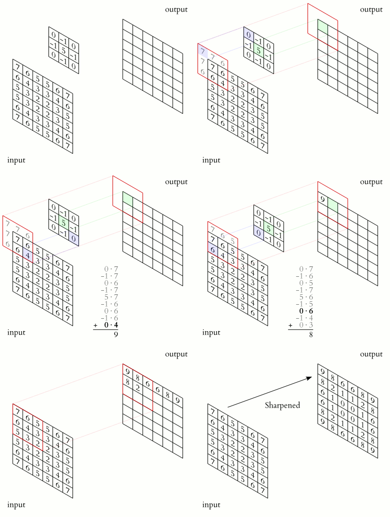
Now you slide this same 3×3 filter across every position in the image. At position (0,0), you compute one output value. Slide one pixel to the right to (0,1), compute another. Keep sliding across and down until you’ve covered the entire 224×224 input, producing a 224×224 output where each value represents the edge strength at that position.
Controlling the Output: Padding and Stride
When we slide that window, we have two important knobs to turn that determine the shape of our output feature map.
1. Padding
If you have a 5×5 image and apply a 3×3 filter, you can only fit the filter in 3 positions horizontally and 3 positions vertically. Your output becomes 3×3. You "shrank" the image by 2 pixels.
If you keep doing this in a deep network, your 224×224 image will vanish into a single pixel after just a few layers! To prevent this, we use Padding. We add "fake" pixels (usually zeros) around the edge of the input.
-
Valid Padding: No padding. The image shrinks.
-
Same Padding: Add just enough zeros so the output is the same size as the input. For a 3×3 filter, we add 1 pixel of padding to every side.
2. Stride
Stride is how many pixels the filter "jumps" each step. * Stride = 1: Move one pixel at a time. High detail, high computation. * Stride = 2: Skip every other pixel. This effectively cuts the output resolution in half (224×224 → 112×112).
In modern architectures, Strided Convolution (Stride=2) is often used instead of Pooling to reduce image size, because the network can learn how to downsample, rather than using a fixed rule like "take the maximum."
Multiple Channels: The 3D Convolution
Real images aren’t just 2D grids; they have depth (Red, Green, Blue). A convolutional filter in the first layer of a CNN is actually a 3D volume.
If the input is 224×224×3, a 3×3 filter is actually 3×3×3. It looks at a 3×3 patch across all three color channels simultaneously. It might learn, for example, that a "vertical edge that is mostly red" is a specific feature it needs to find.
When you have 64 such filters, each one produces one 2D feature map. You stack those 64 maps to create a 224×224×64 output. The next layer’s filters will then be 3×3×64—seeing all the features discovered by the previous layer.
This is the key to why CNNs are so powerful: they aren’t just looking for 2D patterns; they are looking for correlations across multiple "layers" of information.
Building a Convolutional Layer
A convolutional layer contains multiple filters (usually 32-128 in early layers, 256-512 in later layers). Each filter learns to detect a different pattern:
-
Filter 1: Horizontal edges
-
Filter 2: Vertical edges
-
Filter 3: Diagonal edges (top-left to bottom-right)
-
Filter 4: Diagonal edges (top-right to bottom-left)
-
Filter 5: Corners
-
Filter 6-32: Other patterns learned during training
When you apply all 32 filters to a 224×224 RGB input, you get 32 output images (called "feature maps"), each 224×224, each highlighting where a specific pattern appears.
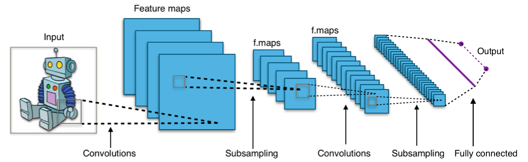
Input: 224×224×3 (height × width × RGB channels) ↓ Apply 32 different 3×3×3 filters (3×3 spatial, across all 3 color channels) ↓ Output: 224×224×32 (height × width × 32 feature maps)
Each of those 32 filters has 3×3×3 = 27 weights (plus 1 bias) = 28 parameters per filter. Total: 32 filters × 28 = 896 parameters for the entire layer.
Compare to the 77 million parameters in a fully connected layer doing the same job. This is why convolution works.
Why This Solves Our Problems
Translation invariance: The same filter detects a cat’s ear whether it’s at (50,50) or (150,100). We learned the pattern once.
Parameter efficiency: Instead of millions of separate weights for every position, we have hundreds of shared weights applied everywhere.
Spatial locality: A 3×3 filter naturally respects that nearby pixels are related—it only looks at local regions.
Hierarchical features: Stack multiple convolutional layers and you get hierarchy for free. Layer 1 detects edges. Layer 2 combines edges into shapes. Layer 3 combines shapes into object parts. Layer 4 combines parts into objects.
From Edges to Objects: The Hierarchy
Let’s trace what happens when you feed a photo of a dog through a convolutional network:
Layer 1 (input: 224×224×3, output: 224×224×64):
Learns edge detectors, color blobs, simple textures. One filter responds to vertical edges, another to horizontal edges, another to red-to-brown gradients. The outputs look like edge maps—abstract, not recognizable as objects yet.
Layer 2 (input: 224×224×64, output: 112×112×128):
Combines edges into shapes. A filter might respond to "corner formed by horizontal and vertical edge". Another responds to "circular boundary". These are still low-level, but starting to look like parts of objects. We also reduce spatial resolution (224→112) because we care more about "what" than "exactly where".
Layer 3 (input: 112×112×128, output: 56×56×256):
Combines shapes into parts. One filter activates for "furry texture bounded by curved edges" (could be part of a dog, cat, or teddy bear). Another responds to "round shape with high contrast" (eye candidate). Another detects "rectangular with parallel lines" (window, door, or book spine).
Layer 4 (input: 56×56×256, output: 28×28×512):
Combines parts into object-specific features. At this level, you have filters that activate specifically for "dog face", "car wheel", "bird wing". The spatial resolution is coarse (28×28) because we don’t need precise localization for classification—we just need to know "this image contains a dog", not "the dog’s nose is at pixel (145, 87)".
Final Layer (global average pooling + fully connected):
Takes the 28×28×512 feature maps and reduces them to 1000 class scores. "I see strong evidence for dog features, weak evidence for cat features, no evidence for airplane features → predict: dog".
This hierarchy isn’t hand-designed. You don’t tell the network "layer 1 learns edges, layer 2 learns shapes". You initialize all the filters with random weights and train with backpropagation, the same as MNIST. The hierarchy emerges because it’s the optimal way to solve the problem given the convolutional structure.
Non-Linearity: Why ReLU is King
A convolution is a linear operation (multiplication and addition). If you stack ten linear layers together, the result is still just one big linear operation. You could mathematically collapse the whole network into a single layer!
To learn complex, non-linear patterns (like "a dog’s ear"), we must inject non-linearity between the layers. We use an Activation Function.
ReLU (Rectified Linear Unit)
In modern CNNs, we almost exclusively use ReLU:
-
Why? It’s computationally "free"—in a shader, it’s just
max(0.0, value). -
Gradient Flow: Unlike the Sigmoid function (which "squashes" values between 0 and 1, causing gradients to vanish), ReLU doesn’t saturate for positive values. This makes deep networks much easier to train.
Batch Normalization: The Stabilizer
As data flows through a deep network, the values can drift—some layers might start outputting very large numbers, while others output tiny ones. This is called Internal Covariate Shift, and it makes training very unstable.
Batch Normalization solves this by "re-centering" the data after each convolutional layer. It ensures that the mean is near 0 and the standard deviation is near 1.
-
During Training: It calculates the mean/std of the current batch.
-
During Inference (Vulkan): These values are pre-calculated and "folded" into the convolutional weights. This means Batch Norm is free at runtime! When you use a model in ONNX Runtime, you don’t even see the Batch Norm layers; they’ve been mathematically merged into the convolutions to save performance.
Receptive Fields: How Deep Patterns See
A critical concept: receptive field. How much of the original image does a neuron in layer 4 "see"?
In layer 1, a 3×3 filter sees exactly 3×3 pixels of the input.
In layer 2, a 3×3 filter sees 3×3 positions of layer 1’s output. But each of those positions came from 3×3 pixels in the input. So layer 2 effectively sees:
Layer 2 receptive field = 3 + (3-1) = 5×5 input pixels
In layer 3, each position sees 3×3 of layer 2, and each layer 2 position sees 5×5 of input:
Layer 3 receptive field = 5 + (3-1) = 7×7 input pixels
By layer 5, a single neuron might see 13×13 or more input pixels, depending on the exact architecture.
This is how deep networks build complex patterns from simple ones. Early layers see small regions and detect simple patterns. Later layers see large regions (because they’re seeing outputs from early layers) and detect complex patterns.
Pooling accelerates this. When we reduce 224×224 to 112×112, each position in the smaller map corresponds to 2×2 region in the larger map. This doubles the receptive field growth rate.
Why Not Just Use Bigger Filters?
You might ask: why not skip the hierarchy and use, say, 11×11 filters in layer 1 to see more context?
Parameters. An 11×11 filter has 121 weights per channel. For a layer with 64 filters processing RGB input:
11×11×3 channels × 64 filters = 23,232 parameters
Compare to two 3×3 layers stacked (which has the same receptive field):
Layer 1: 3×3×3 × 64 = 1,728 parameters
Layer 2: 3×3×64 × 64 = 36,864 parameters
Total: 38,592 parameters
Wait, that’s more parameters! But there’s a critical difference: two layers with ReLU activation in between.
Stack two 3×3 convolutional layers with ReLU between them and you get the same receptive field (5×5 in the input) as one 5×5 layer, but with more non-linearity. The extra ReLU lets the network learn more complex functions. Three 3×3 layers cover the same receptive field as one 7×7, but with three non-linearities instead of one.
This is why modern networks (like VGG, ResNet, MobileNet) use almost exclusively 3×3 and 1×1 convolutions. Larger filters waste parameters without adding representational power.
Pooling and Spatial Reduction
We mentioned reducing 224→112→56→28. Why?
Computational efficiency: A 224×224 image has 50,176 positions. A 112×112 image has 12,544—4× fewer. Pooling cuts computation dramatically.
Translation invariance: If you shift the input image by 1 pixel, max pooling (taking the maximum in each 2×2 region) might produce the same output. The exact position matters less.
Abstraction: For classification, you don’t care if the dog’s eye is at (45,67) or (47,68). You care that there’s an eye somewhere in the upper-middle of the image. Reducing spatial resolution forces the network to learn position-invariant features.
Max pooling takes the maximum value in each small region (typically 2×2) and outputs it. A 2×2 max pooling operation with stride 2 reduces a 4×4 input to a 2×2 output—you take the max of each non-overlapping 2×2 block.
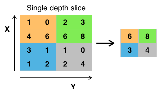
Modern architectures sometimes use strided convolution instead (convolution with stride=2 skips every other position), which is learnable rather than hard-coded like max pooling. But the principle is the same: progressively reduce spatial dimensions while increasing channel depth.
The Pattern: Conv → ReLU → Pool → Conv → ReLU → Pool…
Almost every CNN follows this pattern:
Input Image (224×224×3)
  ↓
[Conv 3×3 → ReLU → Pool] → (112×112×64)
[Conv 3×3 → ReLU → Pool] → (56×56×128)
[Conv 3×3 → ReLU → Pool] → (28×28×256)
[Conv 3×3 → ReLU → Pool] → (14×14×512)
  ↓
Global Average Pool → (1×1×512)
  ↓
Fully Connected → (1000 class scores)
  ↓
Softmax → (probabilities)
Spatial dimensions shrink: 224 → 112 → 56 → 28 → 14 → 1
Channel depth grows: 3 → 64 → 128 → 256 → 512
This trades spatial detail for semantic depth. Early layers answer "where are the edges?" Late layers answer "is there a dog?"
MobileNetV2: Making CNNs Efficient
Standard convolution is expensive. A 3×3 convolution with 512 input channels and 512 output channels requires:
3×3 spatial × 512 input × 512 output = 2,359,296 operations per position
For 28×28 image: 2.36M × 784 = 1.85 billion operations
MobileNetV2 uses a trick called depthwise separable convolution. Instead of one expensive operation, split into two cheaper ones:
Depthwise convolution: Apply 3×3 filter to each channel separately.
Input: 28×28×512 (512 separate channels)
Apply 512 different 3×3 filters (one per channel)
Output: 28×28×512
Cost: 3×3 × 512 = 4,608 operations per position
This captures spatial patterns within each channel but doesn’t mix information across channels.
Pointwise convolution: Apply 1×1 convolution to mix channels.
Input: 28×28×512
Apply 512 different 1×1×512 filters
Output: 28×28×512
Cost: 1×1 × 512 × 512 = 262,144 operations per position
This mixes information across channels but doesn’t look at spatial neighbors.
Total cost: 4,608 + 262,144 = 266,752 operations per position
Compare to standard convolution: 2,359,296 operations per position.
Speedup: 8.8× with minimal accuracy loss.
The MobileNetV2 Block: Inverted Residuals
MobileNetV2 takes this efficiency further with the Inverted Residual Block.
Traditional Residual blocks (like in ResNet) follow a "Wide → Narrow → Wide" pattern. They take a large number of channels, compress them, then expand them.
MobileNetV2 does the opposite: Narrow → Wide → Narrow.
-
Expansion (1×1 Conv): Take the small number of input channels and expand them (usually by a factor of 6). This gives the depthwise convolution more "room" to find patterns.
-
Depthwise (3×3 Conv): Perform the spatial filtering on the high-dimensional data.
-
Projection (1×1 Conv): Compress the data back down to a small number of channels.
Linear Bottlenecks
A subtle but vital detail: the final 1×1 Projection layer in the block does not use ReLU.
Why? If you use ReLU on a low-dimensional space, you lose too much information (it zeros out half the data). By using a linear activation (no activation) at the bottleneck, the network can preserve the complex features it just discovered.
This combination of depthwise separable convolutions, inverted residuals, and linear bottlenecks is what allows MobileNetV2 to run at 60 FPS on your phone while still recognizing thousands of objects correctly.
Why MobileNetV2 Matters for This Tutorial
When you’re implementing inference in Vulkan, you need to know which operations dominate runtime. For MobileNetV2:
Pointwise convolutions (those 1×1 convolutions mixing channels) are matrix multiplications. They’re compute-bound. Optimizing them means maximizing arithmetic throughput—using tensor cores, vectorized instructions, large thread blocks.
Depthwise convolutions (the 3×3 per-channel filters) are memory-bound. Each output value requires reading 9 input values and 9 weights. Optimizing them means improving memory access patterns—coalescing reads, using shared memory, minimizing cache misses.
Understanding the architecture tells you where to focus optimization. If you spend days optimizing ReLU (which is just max(0, x)), you’ll see minimal speedup because ReLU is <1% of runtime. If you optimize the pointwise convolutions, you can get 2-3× faster inference.
This is why we teach the theory before the implementation.
How the Network Learns: Backpropagation Intuition
We’ve talked about what filters do, but how do they get their values? In MNIST, we had a few thousand weights. In MobileNetV2, we have millions. We can’t tune them by hand.
We use Backpropagation combined with Stochastic Gradient Descent (SGD).
The Loss Surface
Imagine the network’s error (Loss) as a mountain range. The "height" at any point is how many images the network got wrong. The "coordinates" (longitude and latitude) are the values of the millions of weights in the network.
When we start, the weights are random. We are standing on a random mountain peak. Our goal is to find the lowest valley—the point where the error is zero.
The Gradient
We take an image (e.g., a dog), feed it forward, and see the result. If the network predicts "car," the Loss is high.
We then calculate the Gradient. The gradient is a mathematical vector that tells us: "If you change weight by a tiny amount, the Loss will go up. If you change weight , the Loss will go down."
Where (eta) is the Learning Rate—how big of a step we take down the mountain.
Training at Scale
In a CNN, the gradient for a filter in layer 10 depends on all the layers after it. Backpropagation "zips" backward from the output to the input, calculating how much each filter contributed to the wrong answer.
This is why training is so slow compared to inference. Inference is just one "Forward Pass" (down the mountain). Training is thousands of forward and backward passes (calculating the slope and taking a step).
Preparing for Success: Data Augmentation
Even the best architecture will fail if the data is poor. If you only show the network photos of dogs on grass, it will learn that "green background = dog." If you show it a dog on a sidewalk, it might predict "grey car."
To prevent this, we use Data Augmentation. During training, we don’t show the network the same image twice. We "mess with it" first:
-
Random Flip: Flip the dog horizontally. It’s still a dog.
-
Random Crop: Zoom in on the tail or the ears. The network learns that parts of a dog are just as important as the whole.
-
Color Jitter: Change the brightness, contrast, and saturation. A dog in the sun is the same as a dog in the shade.
-
Rotation: Rotate the image by a few degrees.
By the time training is finished, the network has seen millions of variations of dogs, making it incredibly robust to real-world camera noise and lighting conditions.
The Final Decision: Softmax and Cross-Entropy
At the very end of our millions of multiplications, the network spits out 1000 numbers (one for each ImageNet class). These are called Logits. They might look like this:
-
Dog: 14.2
-
Cat: 8.5
-
Car: -2.1
These aren’t very useful to a human. We want Probabilities that add up to 100% (1.0).
The Softmax Function
To turn Logits into Probabilities, we use the Softmax function:
Where is the logit for class .
-
The Power of : Using the exponential function means that the highest logit gets the "lion’s share" of the probability. It "rewards" the winner and "punishes" the losers.
-
Normalization: The denominator ensures that all the probabilities add up to exactly 1.0.
Cross-Entropy Loss
During training, we need to compare these probabilities to the "Ground Truth" (e.g., if the image is a dog, the probability should be 1.0 for Dog and 0.0 for everything else). We use Cross-Entropy Loss:
If the network is 100% confident in the correct answer, the loss is 0. If it’s confident in the wrong answer, the loss becomes nearly infinite. This creates a very "steep" mountain for the gradient descent to follow, leading to fast learning.
What You’ve Learned
You now understand:
-
Why fully connected networks fail for images: Too many parameters, no translation invariance, ignore spatial structure
-
What convolution is: Shared weights applied everywhere, detecting patterns regardless of position
-
How CNNs build hierarchies: Edges → shapes → parts → objects through stacked layers
-
Why 3×3 filters dominate: Efficient parameters, stackable for large receptive fields, added non-linearity
-
What pooling does: Reduces spatial dimensions, increases translation invariance, cuts computation
-
How MobileNetV2 works: Depthwise separable convolutions trade accuracy for efficiency
-
Why architecture matters for implementation: Knowing what operations dominate tells you what to optimize
Next, we’ll implement this. You’ll build a complete image classification pipeline: loading images, preprocessing them, running inference with ONNX Runtime, and displaying results. Then we’ll add GPU acceleration, threading for responsiveness, and real-time camera input.
But now you understand what you’re implementing and why it works. The code is just the expression of these concepts.